The display below shows an interactive guided tour of the ArcMap program. Only the relevant features of ArcMap will be discussed. The disply uses VCR-like controls to allow you to navigate through the presentation. Click on the left arrow button to move backward and the right arrow button to move forward.
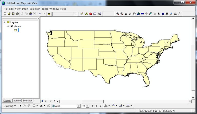
In the next part of this module we will take you through a simple emergency application of ArcMap. Please open the ArcMap software on your machine. This tutorial will walk you through the application. The presentation is designed to lead you through the necessary steps. There are probably for or five different ways to accomplish each of the steps in the tutorial. We have selected the one that is the simplest and easiest to follow. You can take time on your own to learn more sophisticated ways ap manipulating the ArcGIS programs. You should be able to recreate the screens in the tutorial on your instance of ArcMap. If you get stuck at any point, you can back up to the last point in the tutorial where your display matched the tutorial. The image below shows the ArcMap initial screen which is our beginning point.
Load Data
The first task is to load spatial data into ArcMap. The data is contained in a shapefile, which is really a set of files. Normally a map is created with multiple shapefiles. Shapefiles are arranged in layers such that the lowest layers, called base layers or basemap, may be occluded all or in part by the upper layers. Generally a shapefile is used to represent a common feature or theme. The map of the United states below was created with shapefiles for the Oceans, Canada, Mexico, US Background, States, Highways, Water, and Cities from bottom to top. Part of the process of creating a good map has to do with layer selection and level, colors and other display factors.
Definition:
basemap A map depicting background reference information such as landforms, roads, landmarks, and political boundaries, onto which other thematic information is placed.
shapefile A vector data storage format for storing the location, shape, and attributes of geographic features. A shapefile is stored in a set of related files and contains one feature class.
A shapefile as defined by ESRI is a cluster of files pertaining to a spatial construct. A shapefile can be of type
point - each shapefile entry describes an entity at a location in space: longitude, latitude and optionally altitude.
polyline - each shapefile entry describes a sequence of straight lines
polygon - each shapefile entry describes a closed area
Point shapefiles are good for representing things that are at single locations e.g. fire hydrants, buildings, events, etc. Polyline shapefiles are used to represent roads, borders and other like geometric entities. Polygon shapefiles are good for representing, countries, states, counties, parks, building footprints and other elements where a representation of an area extent is desired.
In the map above the Oceans, Canada, Mexico, US Background States, and Water were represented in polygon shapefiles. Highways were represented in a polyline shapefile and Cities were represented in a point shapefile.
The accompanying ESRI document shapefile describes the specification of shapefiles.
The table below shows the components of a polygon shapefile that contains the representations for all of the states of the United States.
Our first step is to download the states shapefile into a local directory on your computer. To do this:
Create a directory on your computer named GISData
For each of the component files in the table above (states.shp, states.shx, stated.dbf, states), right click on the file name.
Select "Save Target As..." from the popdown menu.
Navigate to the GISData directory in the Save As dialog form
Click the Save button
Displaying the Layer
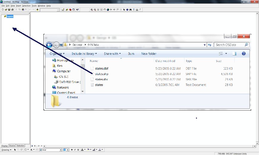
Use the Windows file explorer to navigate to the GISData directory. Click on the states.shp file and drag and drop it onto the Layer area of ArcMap (the leftmost tall, thin area) as shown below. Note: you may get a popup warning you about projection coordinate systems. Ignore this for now.
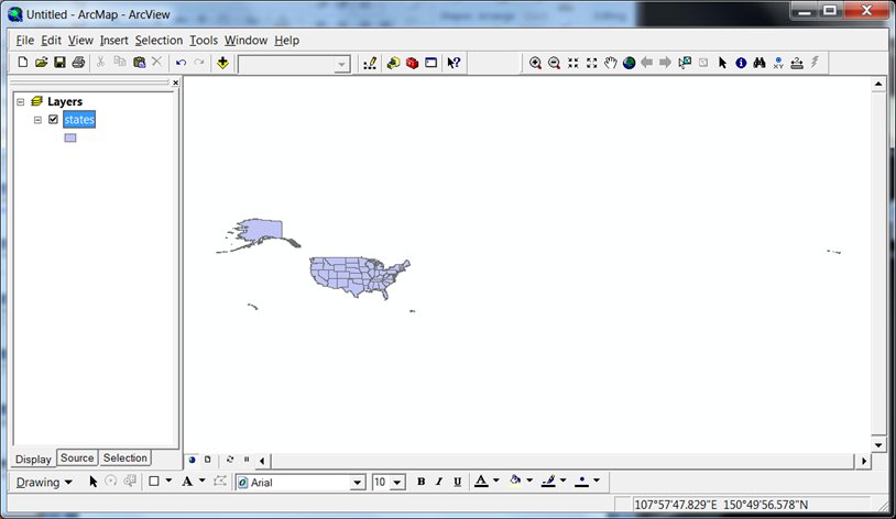
What you should get is something that looks like the display below. There are a couple of problems with this display. First, the color used to fill the state polygons is usually not very aesthetic. Second, the display is at a scale that is not desired.
Focus on the area to the left of the display where you dragged the states shapefile. Under the shapefile name is a rectangle filled with a solid color.
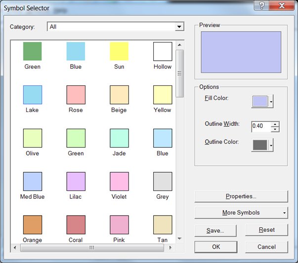
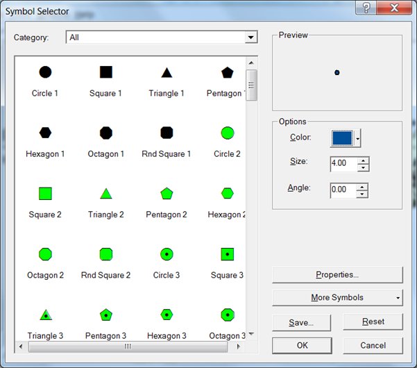
If you click on the rectangle, the Symbol Selector form shown to the right will pop up.
This form will allow you to change the representations for the polygons in the shapefile. At the top of the form are solid color fills. If you scroll down, you will see fills using hatched and other patterns commonly used in maps. Clicking on a color will select that color for your polygons.To the right is a preview pane that shows the effect of your changes. Below the pane is a selector that will change the border representation for the outline of each polygon. You can select the border thickness and/or color.
For this example we will change the color of the polygons to yellow and leave the outline width unchanged (.04, Black).
When you are satisfied with your modifications, click the OK button and the changes will be applied to the ArcMap display.
Exercise:
When you have time, explore the options associated with the display of polygons. In particular, nothe the effects of using Hollow fill and changing the properties of Outline. Also look at the More Symbols feature which allows a user to load representations from other sets and upload custom representations.
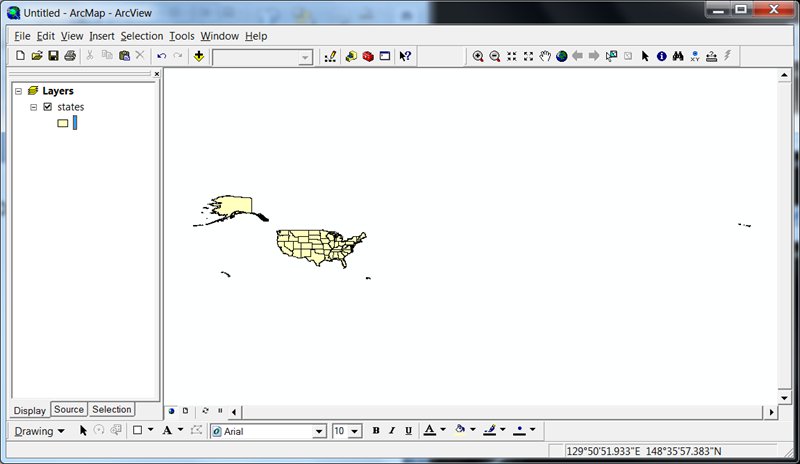
If all has gone well, you should have the ArcMap display shown below.
Next we need to take care of the scale. There are two ways to do this:
Select the magnifying glass tool with the plus sign on the toolbar . Drag the cursor across the rectangular area that includes the continental United States.
Use the Zoom In tool . The Zoom In tool operates at the center of the display.
In both of the strategies above, you will probably have to make some minor corrections along the way. You can make these corrections with:
The Magnifier Glass with the Minus Tool zooms out centered around the selected area.
The Pan Tool that moves the display left, right, up or down.
The Zoom Out Tool does the opposite of Zoom In Tool.
The Back and Forward Tool Buttons change the display to the previous display.
When you are hopelessly lost, the Globe Tool changes the map display to the original extent.
Your goal is to create a display of the continental United States that looks reasonably like the one shown below.
Exercise:
Make sure that you are facile with the map navigation tools presented in the previous section. As a test, practice zooming in on particular states or regions.
Multiple Layers
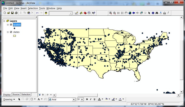
The table below shows the components of a point shapefile that contains the representations for all of the historical earthquakes that occurred in the states of the United States.
As with the states shapefile, our first step is to download the quakes shapefile into the same local directory (GISData) that you created before on your computer. To do this:
For each of the component files in the table above (quakes.shp, quakes.shx, quakes.dbf), right click on the file name.
Select "Save Target As..." from the popdown menu.
Navigate to the GISData directory in the Save As dialog form
Click the Save button
The process of displaying the Layeris identical to the states layer. Use the Windows file explorer to navigate to the GISData directory. Click on the quakes.shp file and drag and drop it onto the Layer area of ArcMap (the leftmost tall, thin area) as shown below. Note: you may get a popup warning you about projection coordinate systems. Ignore this for now.
You may have accidentally created a map where the states layer is on top of the quakes layer. To correct this simply drag the quakes layer on top of the states layer in the Layer window.
Just as with polygons, ArcMap has selected a default representation for the points on our shapefile.
To change the representations for the points, click on the point below the shapefile name in the Layer window. The form shown to the right will pop up. If you scroll down, you will see all sorts of point shape representations. There are not only geometric representations but representations from international icon sets and other specialized representations. The More Symbols button will let you load representations from other sets or your own custom created representations.
To the right is a preview pane that shows the effect of your changes. Below the pane is a selector that will change the border representation for the outline of each polygon. Clicking on the color will allow you to select a custom color for your shape. You can select the size, angle and/or color.
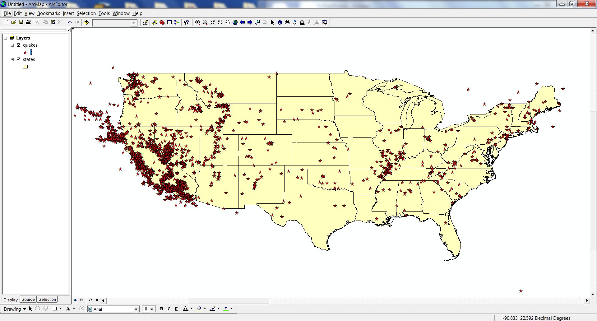
For this example we will change the symbol to the "Star 3" shape its Color to red and Size to 10 pixels.
When you are satisfied with your modifications, click the OK button and the changes will be applied to the ArcMap display.
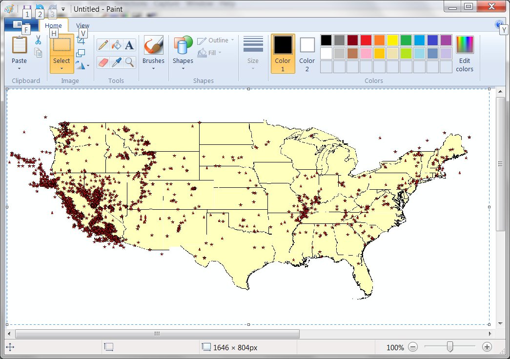
The map that you get should look like the map displayed below.
This display is quite good for assessing the patterns of earthquakes in the US. However, we would like to get information about each of the earthquakes.
Accessing Map Data
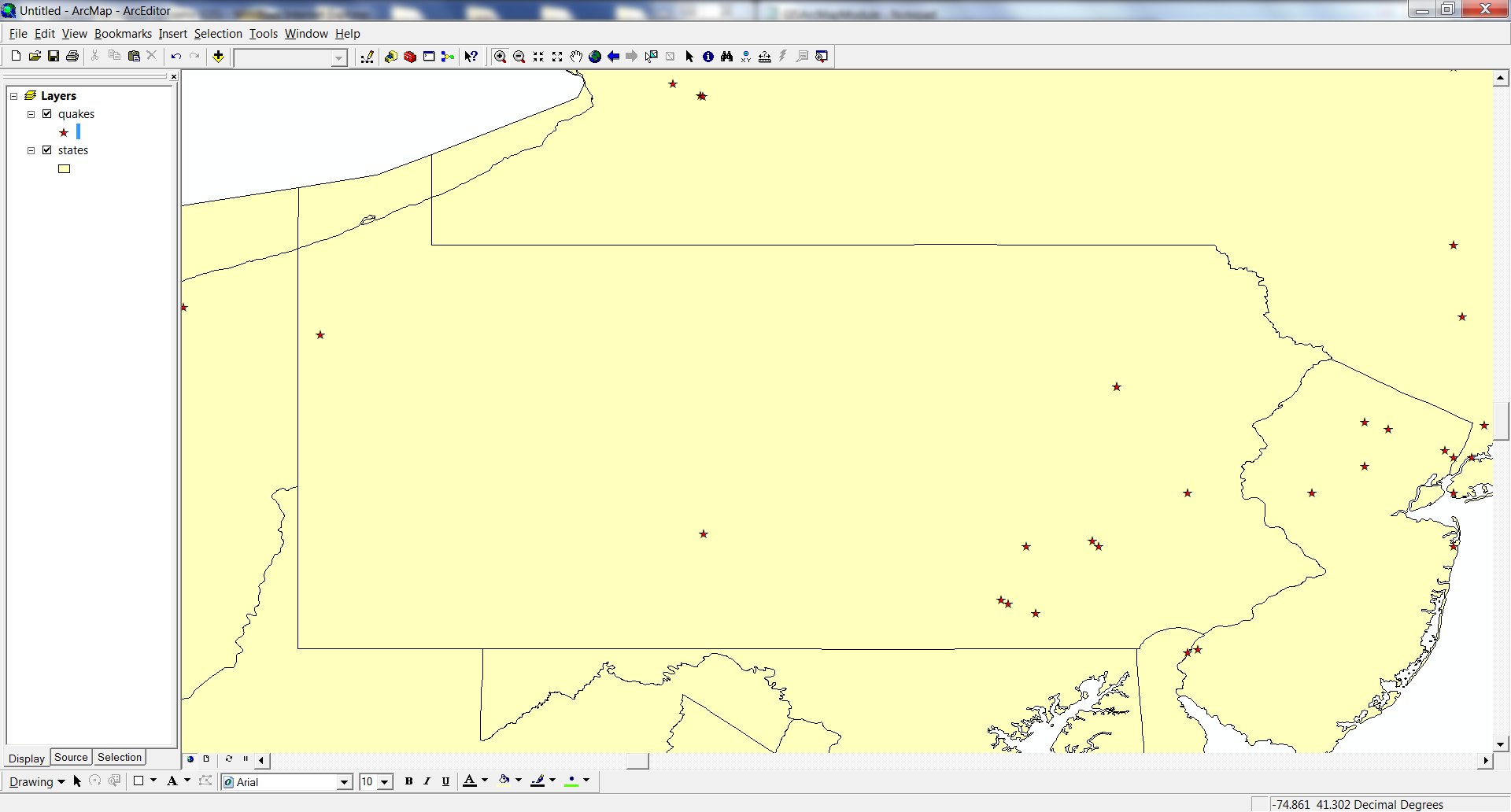
Zoom into Pennsylvania using one of the methods from our previous discussion. You should get something like the map below.
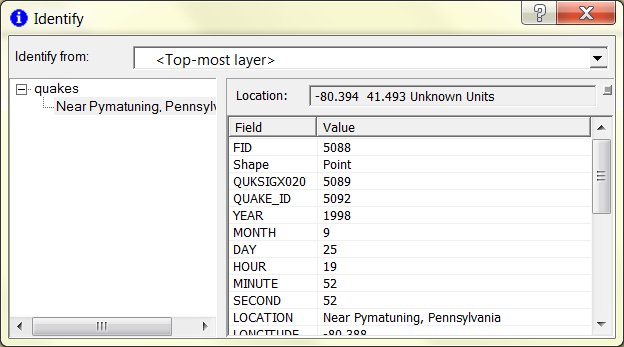
Click on the Identify Tool on the toolbar. A popup form display like the one below should appear.
Click on any of the stars (earthquakes) and the data from that earthquake will appear. The data includes the location of the earthquake, time, size and other relevant information.
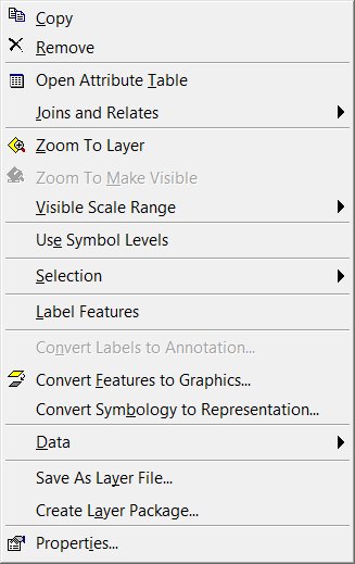
The technique for accesssing layer information presented above is good for finding out about a particular or a few earthquakes. To access all of the information about all of the earthquakes, go to the Layers window and right-click on the name of the earthquake layer (quakes). A menu like the one shown below will pop up. Select the "Open Attribute Table" option.
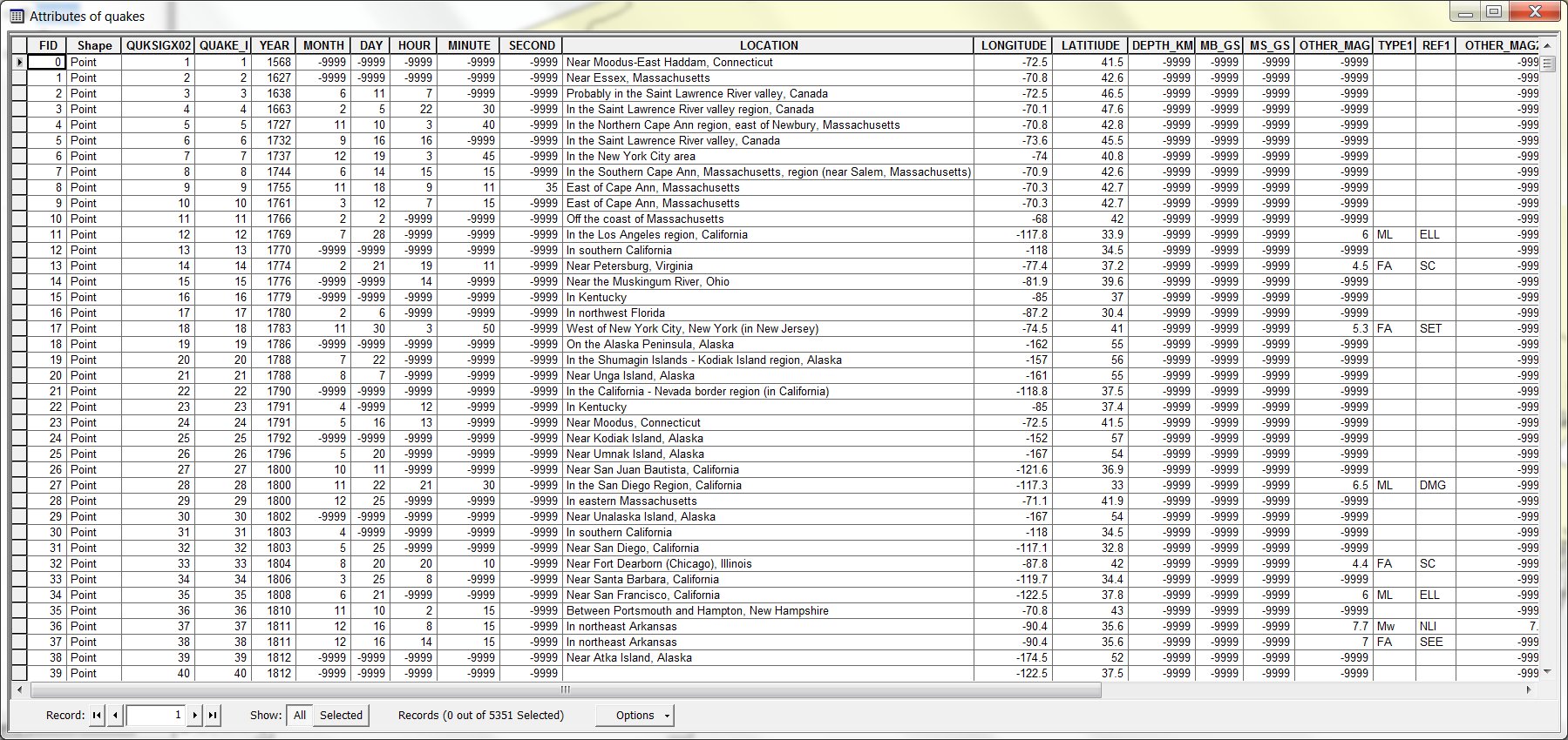
A spreadsheet-like window will open up with all of the data for all of the entries in the layer. This table behaves much like a spreadsheet (i.e. you can sort, navigaate, select, etc.).
Saving Map Documents
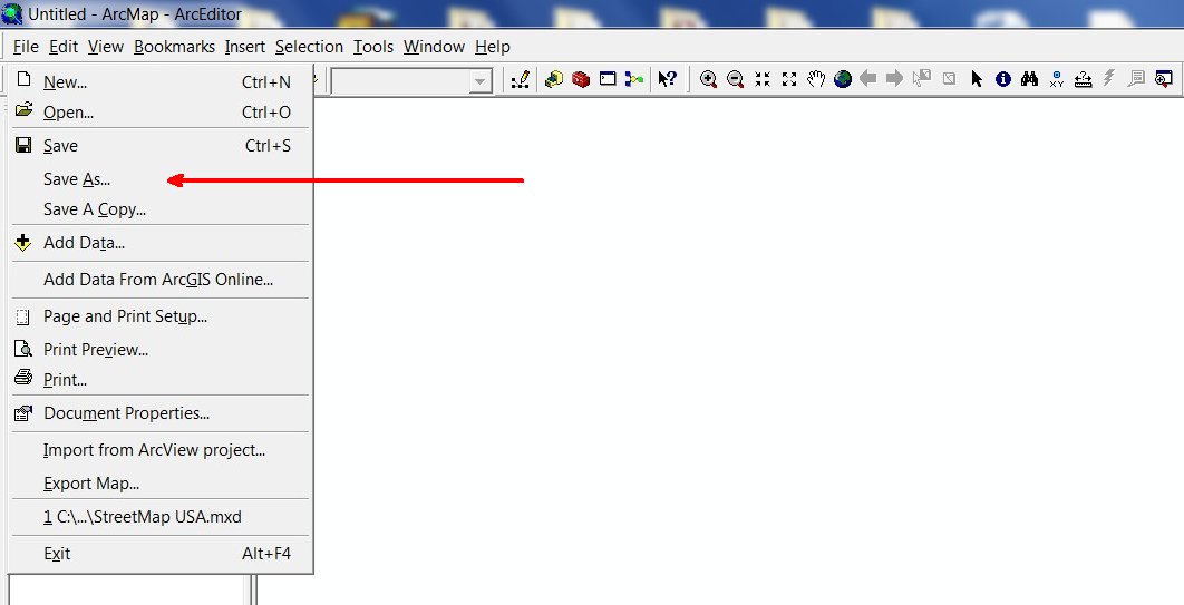
To save a map in the form that you have built it, click on the "File" label in the menu bar. In the popdown menus as shown below, click on the "Save As" option. A standard Windows "Save As" form will appear. Navigate to the desired directory (GISData), enter a name and save the map as an ArcMap Document. The ArcMap file will have an .mxd extension. You can open this document at any later time and arrive back at the map state when you saved it.
Exporting Map Images
To save an image of the current map in the form that you have built it, click on the "Edit" label in the menu bar. In the popdown menu, click on the "Copy Map to Clipboard" option. This will copy a bitmap image of the map to Windows shared memory. From here you can paste the map into any Windows compatible program (Word, Powerpoint, Excel, Adobe, etc.). We recommend copying the map into a graphics program such as the Microsoft Paint program or Adobe Photoshop. Simply open up the Paint program. Go to its "Edit" menu item and click on the "Paste" option. The result should be an image of the map within the program as shown below.
The reason that we recommend using a graphics program first is that we can now use graphical operations to, enhance, recolor, resize, clip, title and do numerous other operations on our map. But, perhaps most importaantly, we can save the map to a popular image file format such as JPEG, GIF, or PNG for use in a website or other application.
Layers
As we have seen, adding shapefiles to a map creates layers of information. Many times we want to create multiple maps that are derivatives of the same basemap. In this case, it is advantageous to build an ArcMap Document that contains all of the layers that we are going to use. Note that to the left of each layer name in the Layers list is a checkbox. That checkbox controls whether the llayer is visible in the current view. We can create multiple versions of the same map by displaying different combinations of layers. The map animation below shows a basemap of the states layer with layers for Interstates, airports and amtrak stations. The animation progresses with each map displaying an additional layer.
The additional shapefile data to produce the above maps are contained in the files below.
Basemap layers serve as a basis for all of the layers that are added above them. Selection of a basemap layer should be consider two factors:
The layer should be relevant to the problem at hand. In other words, the granularity of the base map should reflect the level of analysis we are performing: International, National, Regional, State, County, Local, etc.
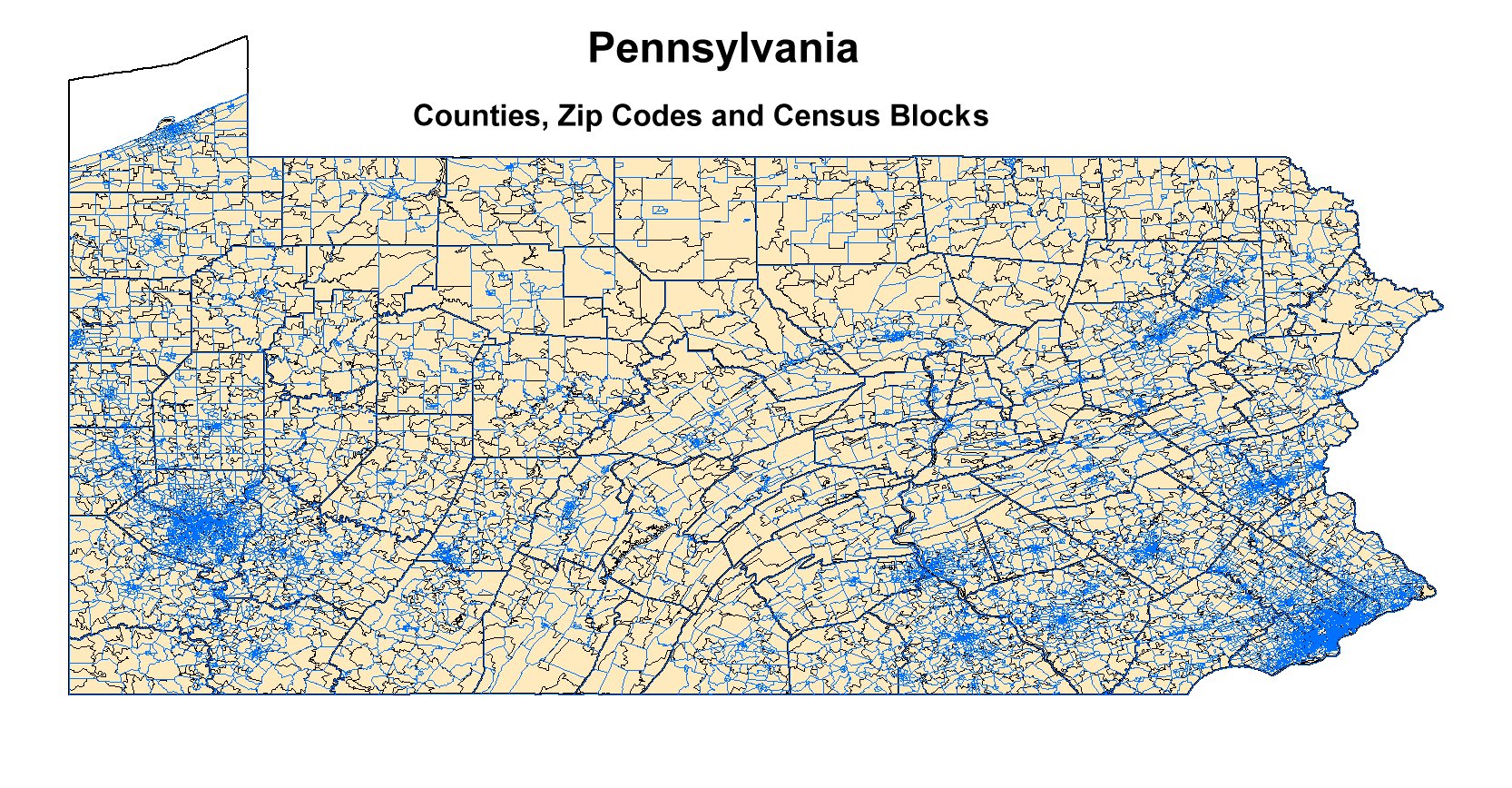
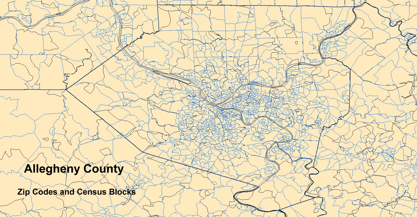
The basemap layer should be useful for any new information that we might wish to collect, analyze and display. For example, we may wish to collect information on citizens who would need assistance for evacuation. County level information would be useful for planning. Information at the Zip Code or Census block level would be useful in identifing which emergency agency would respond.
The maps below show several common levels of basemap data that are readily available.
The shapefile data for the above maps are accessible through the table below.