NPHS 1530: Analytics

Reliability

FACTORS AFFECTING RELIABILITY

In the preceding sections we have treated the reliability of a component and thus a system, as a constant. In reality, the reliability of a component may change with a number of factors such as temperature, pressure, age and duty cycles. The reliability of most components declines with time and other factors. There are some devices, however, where reliability may increase over some period of use. Most treatments of reliability deal with its change over time. Since the age, number of duty cycles and other use factors of a component are typically highly correlated with time, this approach seems the most appropriate. Reliability has previously been defined as the probability that a system or component will operate in the next instant. This ignores the fact that the system may have been operating for a period of time, T. It is generally easier to think in terms of failure probabilities, so we will define a component's reliability as the complement of the probability that the system will fail in the next instant, given that the system has operated for T units of time.  This failure probability is often referred to as the Instantaneous Failure Rate (IFR) or the Hazard Rate (HR). r = 1 - Pr( Failure / T ) The failure probability is a conditional probability and thus can be expressed as the quotient of the component's failure probability density function over time, f(t), and the probability the component will fail at a time later than T, Pr(t=T). Pr( Failure / T ) = { f(t) } / {Pr( t >= T ) } The component's failure probability, Pr(t=>T), can easily be derived from the component's failure probability density function, f(t). What we need is a failure probability density function that has the failure pattern for the component in question. The most commonly used failure probability density function is the exponential function given as:

f(t) =

and plotted below.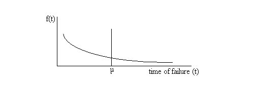 The Exponential Failure Probability Density Function The failure probability density function has a mean of μ. In reliability analysis, we call this figure the mean life of the component or its Mean Time Before Failure (MTBF). Many component manufacturers test the devices (components) they build and report the MTBF for those components as part of their product specifications. The area under the failure probability density function, f(t) may be interpreted as the proportion of a population of components that has failed within a certain time, t. This is how the density function is generated from test data. The actual probability density function generated from test data is a complex function and thus would have little utility in calculations. To simplify our calculations, we approximate the actual density function with the exponential function.

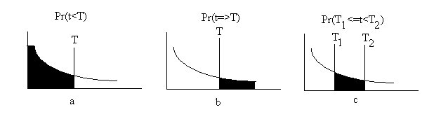The probability that a component will fail within some time, T, Pr(t << T), is defined as the area under the failure probability density function f(t), from zero to time T which may be found by the integral:

Pr( t < T ) =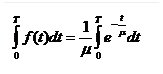

This probability is shown in above.

The value of this integral is:

Pr( t < T ) =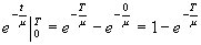

The probability of a component lasting beyond some time, T, is the integral of the probability density function from T to infinity. This probability is shown in the middle Figure above.

Pr( t >= T ) =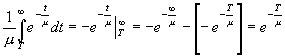

Since the two formulas above are mutually exclusive, collectively exhaustive and, thus, complementary probabilities:

Pr( t < T ) + Pr( t >= T ) = 1

We can also develop the probability of a component failing within a certain time period, say between times T1 and T2. See the third image in the figure above.

Pr( T1  <= t < T2 ) = Pr( t >= T1  ) - Pr( t  >= T2 ) = e-T1/μ - e-T2/μ

or

Pr( T1  <= t < T2 ) = Pr( t < T2  ) - Pr( t  <= T1 ) = 1 - e-T2/ μ - [ 1 - e-T1/μ]

or

Pr( T1  <= t < T2 ) = 1 - Pr( t < T1  ) - Pr( t  >= T2 ) = 1 - [ 1 - e-T1/μ - e-T2/μ]

As an example, consider a light emitting diode (LED) display. Typical LED displays have a mean life, or MTBF, of 100,000 hours. We may be interested in assessing the likelihood of a display failing prematurely, say, within 50,000 hours of being placed into service. This probability is found using the Formulas developed. Values for the exponential function are presented in the Tables. The solution of the formula for this example is:

Pr( T < 50,000 ) = 1 - e-50,000/100,000 = 1 - e-.5 = 1 - .6065 = .3935

Thus 39.35 percent of the LED displays fail within their first 50,000 hours of operation.

Suppose also that we have a policy of automatically replacing these LED display components after 125,000 hours of service. Certain of the components will still be operating at that time and have life remaining in them.  We would like to estimate the percentage of components that will be operating at (or will fail after) 125,000 hours of service. We can assess this percentage by using Formula 8.19.

Pr( t >= 125,000 ) = e-125,000/100,000 = e-1.25  = .2865

For our LED displays with mean lives of 100,000 hours, 28.65 percent of the displays will last longer than 125,000 hours in service.

Finally, in order to have the greatest utility, we expect the majority of the LED displays to last between 90,000 and 110,000 hours of service. Actually we expect them to fail between 90,000 and 110,000 hours. The percentage of the components that fall into this category are:

Pr( 90,000 <= t < 110,000 ) = e-90,000/100,000 - e-110,000/100,000   = e-.9 - e-1.1   = .4066 - .3328   = .0737

In this instance only 7.37 percent of the components have lives within 10,000 hours of the mean life. Returning now to the Instantaneous Failure Rate (IFR), we can develop its formula as: Pr( Failure / T ) =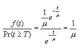

Note that this formulation results in the IFR being a constant. Thus, the IFR and the reliability of a component do not change over the life of the component. This is in line with our previous use of reliability, but does not reflect the reality that some types of components become less reliable with time. This problem can be overcome by using a different probability density function to model the failure pattern of the component. The Weibul Probability Distribution The formula below gives the equation for the WeibulInstantaneous Failure Rate. Pr( Failure / T ) = k * z-k * Tk - 1 Note that if we use the Weibul distribution, the Instantaneous Failure Rate becomes a function of time. The constants k and z are selected to match the Weibul approximation to the component failure test data. The Weibul distribution is actually a parent distribution of the exponential distribution. With k set to one and z = 1/μ , the Weibul distribution becomes the exponential distribution. Values of k <<1 result in a reliability that increases over time. Values of k >1 result in reliabilities for the Weibul distribution that decrease over time. The effects of the value of k on reliability are shown below. IFR for Various Weibul Values of k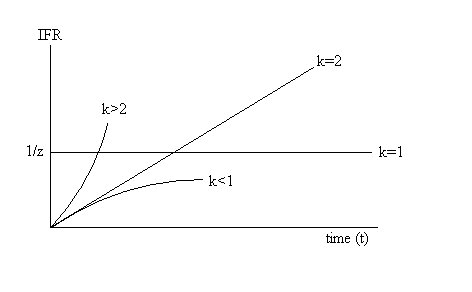

NETWORK RELIABILITY Technically, it is confusing to speak of the reliability of a network. From the user's perspective, he or she is only interested in the integrity of the path(s) between user's location and the destination with which he or she is attempting to communicate. This, as we have seen, is a function of the inherent reliability of the links and nodes that the user is using as well as the number of alternative paths available for communication. Portions of the network that he or she are not using do not affect the individual user's reliability considerations. If we consider all of the users of the network, we might be able to think about an average reliability, or similar measure for all the components of the network. This assumes that each component of the network plays an equal part in the conveyance of network traffic, the traffic between all pairs of users is identical or the traffic on each link is the same, assumptions that are seldom valid.  Other design and operational factors such as level of traffic, routing, directionality of links, etc. have an impact on how network reliability might be calculated. The Figure below shows an early topology of ARPAnet, the communications network sponsored by the Advanced Research Projects Agency of the Department of Defense. As you can see the reliability of the connection between Bell Telephone Laboratories (BTL) and Bolt, Beranek and Newman (BBN) is due mainly to the direct link between these two locations. However, there are also alternative paths between these sites (i.e. BTL - DC -HU - BBN, BBN, BTL - ARPA - UI - MIT -BBN, and many others) that add reliability to the connection. 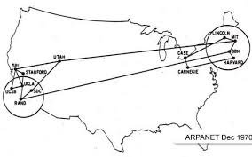ARPAnet Topology Circa 1970 Often in design we make the simplifying assumption that all of the network components (links, nodes, etc.) have the same reliability. This neatly streamlines the calculation. Additionally, the reliability of a single path becomes a function of the number of links, nodes and other network components traversed. R{path} = rc where r = the component reliability and c = the number of path components.  If all of the paths are independent, the reliability between two points in the network is the parallel combination of these paths.

Copyright © 2011 - 2020 Ken Sochats